CellMCD
In this notebook we analyze the covariance of the TopGear dataset using the cellwise minimum covariance determinant which can handle NAs.
Imports
[1]:
import pandas as pd
import matplotlib.pyplot as plt
import numpy as np

from robpy.datasets import load_topgear
from robpy.preprocessing import DataCleaner
from robpy.covariance.cellmcd import CellMCD

%load_ext autoreload
%autoreload 2
Load and preprocess the data
To preprocess the data, we run DataCleaner, as this should always be done before the cellwise analysis. We additionally remove the variable Verdict and take log-transforms of the skewed variables.
[2]:
data = load_topgear(as_frame=True)
car_models = data.data['Make'] + data.data['Model']

cleaner = DataCleaner().fit(data.data)
clean_data = cleaner.transform(data.data)
clean_data = clean_data.drop(columns=['Verdict'])
for col in ['Displacement', 'BHP', 'Torque', 'TopSpeed']:
    clean_data[col] = np.log(clean_data[col])
clean_data['Price'] = np.log(clean_data['Price']/1000)

car_models.drop(cleaner.dropped_rows["rows_missings"],inplace=True)
car_models = car_models.tolist()
clean_data.head()
[2]:
| Price | Displacement | BHP | Torque | Acceleration | TopSpeed | MPG | Weight | Length | Width | Height | |
|---|---|---|---|---|---|---|---|---|---|---|---|
| 0 | 3.056357 | 7.376508 | 4.653960 | 5.463832 | 11.3 | 4.744932 | 64.0 | 1385.0 | 4351.0 | 1798.0 | 1465.0 |
| 1 | 2.718331 | 7.221105 | 4.653960 | 4.553877 | 10.7 | 4.753590 | 49.0 | 1090.0 | 4063.0 | 1720.0 | 1446.0 |
| 2 | 3.433826 | 7.192182 | 4.584967 | 4.521789 | 11.8 | 4.663439 | 56.0 | 988.0 | 3078.0 | 1680.0 | 1500.0 |
| 3 | 4.882764 | 8.688622 | 6.248043 | 6.124683 | 4.6 | 5.209486 | 19.0 | 1785.0 | 4720.0 | NaN | 1282.0 |
| 4 | 4.955792 | 8.688622 | 6.248043 | 6.124683 | 4.6 | 5.209486 | 19.0 | 1890.0 | 4720.0 | NaN | 1282.0 |
CellMCD
[3]:
cellmcd = CellMCD()
cellmcd.fit(clean_data.values)
[3]:
CellMCD()In a Jupyter environment, please rerun this cell to show the HTML representation or trust the notebook.
On GitHub, the HTML representation is unable to render, please try loading this page with nbviewer.org.
CellMCD()
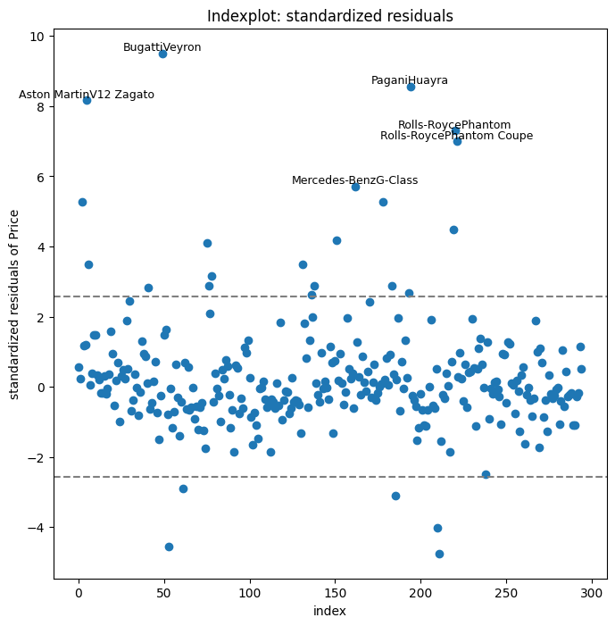
We focus on the variable Price and make several diagnostic plots.
[4]:
variable = 0
variable_name = "Price"
cellmcd.cell_MCD_plot(
    variable=variable,
    variable_name=variable_name,
    row_names=car_models,
    plottype="indexplot",
    annotation_quantile=0.9999999
)
plt.show()
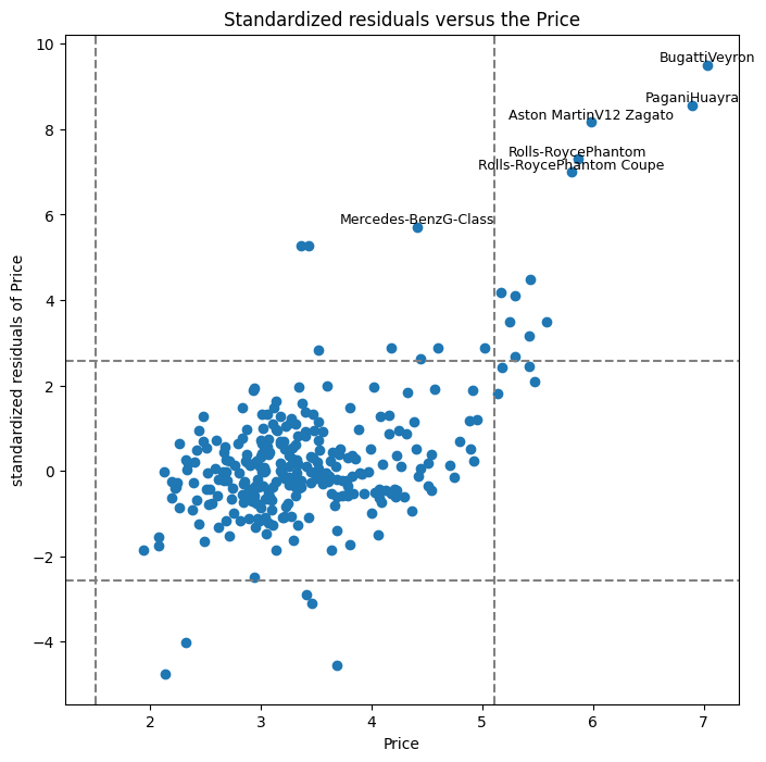
[5]:
cellmcd.cell_MCD_plot(
    variable=variable,
    variable_name=variable_name,
    row_names=car_models,
    plottype="residuals_vs_variable",
    annotation_quantile=0.9999999
)
plt.show()
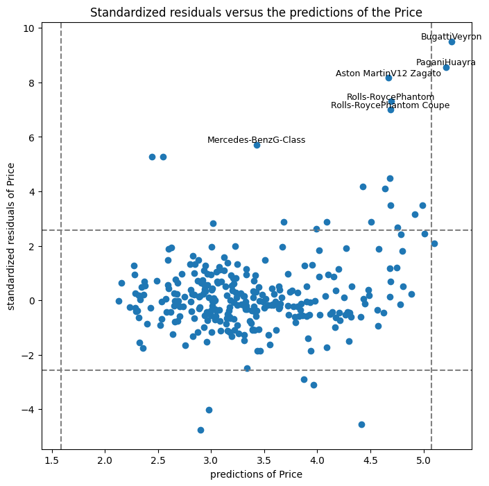
[6]:
cellmcd.cell_MCD_plot(
    variable=variable,
    variable_name=variable_name,
    row_names=car_models,
    plottype="residuals_vs_predictions",
    annotation_quantile=0.9999999
)
plt.show()
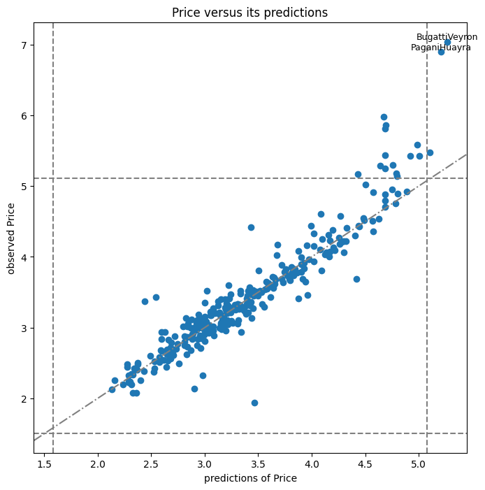
[7]:
cellmcd.cell_MCD_plot(
    variable=variable,
    variable_name=variable_name,
    row_names=car_models,
    plottype="variable_vs_predictions",
    annotation_quantile=0.99999
)
plt.show()
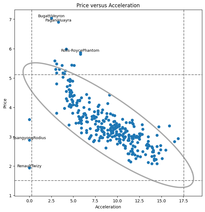
Next we look at the interaction between the variable Price and the variable Acceleration.
[8]:
second_variable = 4
second_variable_name = "Acceleration"
cellmcd.cell_MCD_plot(
    second_variable,second_variable_name,car_models,variable,variable_name,"bivariate",
    annotation_quantile=0.999999
)
plt.show()