TopGear Data
This notebook demonstrates most of the functionality offered by the RobPy package through an application to the TopGear dataset. Utility functions and univariate estimators are not demonstrated separately, as they are mostly implemented as helpers to the multivariate estimators.
Imports
[1]:
import json
import matplotlib.pyplot as plt
import numpy as np

from robpy.datasets import load_topgear
from robpy.preprocessing import DataCleaner, RobustPowerTransformer, RobustScaler
from robpy.covariance import FastMCD, OGK
from robpy.pca import ROBPCA
from robpy.outliers import DDC
from robpy.regression import MMRegression
from robpy.univariate import adjusted_boxplot

%load_ext autoreload
%autoreload 2
Load data
RobPy has a dataset module which allows the user quick access to a few common datasets used in robust statistics literature. In this demo, we will work with the TopGear dataset.
[2]:
data = load_topgear(as_frame=True)

print(data.DESCR)
.. _topgear_dataset:

TopGear dataset
--------------------

**Data Set Characteristics:**

- Number of Instances: 297
- Number of Attributes: 32 (13 numeric, 19 categorical)
- Attribute Information:
    * Make (str): the car brand.
    * Model (str): the car model.
    * Type (str): the exact model type.
    * Fuel (str): the type of fuel ("Diesel" or "Petrol").
    * Price (float): the list price (in UK pounds)
    * Cylinders (float): the number of cylinders in the engine.
    * Displacement (float): the displacement of the engine (in cc).
    * DriveWheel (str): the type of drive wheel ("4WD", "Front" or "Rear").
    * BHP (float): the power of the engine (in bhp).
    * Torque (float): the torque of the engine (in lb/ft).
    * Acceleration (float): the time it takes the car to get from 0 to 62 mph (in seconds).
    * TopSpeed (float): the car's top speed (in mph).
    * MPG (float): the combined fuel consuption (urban + extra urban; in miles per gallon).
    * Weight (float): the car's curb weight (in kg).
    * Length (float): the car's length (in mm).
    * Width (float): the car's width (in mm).
    * Height (float): the car's height (in mm).
    * AdaptiveHeadlights (str): whether the car has adaptive headlights ("no", "optional" or "standard").
    * AdjustableSteering (str): whether the car has adjustable steering ("no" or "standard").
    * AlarmSystem (str) whether the car has an alarm system ("no/optional" or "standard").
    * Automatic (str) whether the car has an automatic transmission ("no", "optional" or "standard").
    * Bluetooth (str) whether the car has bluetooth ("no", "optional" or "standard").
    * ClimateControl (str) whether the car has climate control ("no", "optional" or "standard").
    * CruiseControl (str) whether the car has cruise control ("no", "optional" or "standard").
    * ElectricSeats (str) whether the car has electric seats ("no", "optional" or "standard").
    * Leather (str) whether the car has a leather interior ("no", "optional" or "standard").
    * ParkingSensors (str) whether the car has parking sensors ("no", "optional" or "standard").
    * PowerSteering (str) whether the car has power steering ("no" or "standard").
    * SatNav (str) whether the car has a satellite navigation system ("no", "optional" or "standard").
    * ESP (str) whether the car has ESP ("no", "optional" or "standard").
    * Verdict (float) review score between 1 (lowest) and 10 (highest).
    * Origin (str) the origin of the car maker ("Asia", "Europe" or "USA").

- Creator: BBC TopGear
- Source: https://rdrr.io/cran/robustHD/man/TopGear.html

**Data Set Description:**
The data set contains information on cars featured on the website of the popular BBC television show Top Gear.
The data were scraped from http://www.topgear.com/uk/ on 2014-02-24. Variable Origin was added based on the car maker information.
The DESCR attribute of the data object contains all metadata and a description of the dataset.
[3]:
data.data.head()
[3]:
| Make | Model | Type | Fuel | Price | Cylinders | Displacement | DriveWheel | BHP | Torque | ... | ClimateControl | CruiseControl | ElectricSeats | Leather | ParkingSensors | PowerSteering | SatNav | ESP | Verdict | Origin | |
|---|---|---|---|---|---|---|---|---|---|---|---|---|---|---|---|---|---|---|---|---|---|
| 0 | Alfa Romeo | Giulietta | Giulietta 1.6 JTDM-2 105 Veloce 5d | Diesel | 21250.0 | 4.0 | 1598.0 | Front | 105.0 | 236.0 | ... | standard | standard | optional | optional | optional | standard | optional | standard | 6.0 | Europe |
| 1 | Alfa Romeo | MiTo | MiTo 1.4 TB MultiAir 105 Distinctive 3d | Petrol | 15155.0 | 4.0 | 1368.0 | Front | 105.0 | 95.0 | ... | optional | standard | no | optional | standard | standard | optional | standard | 5.0 | Europe |
| 2 | Aston Martin | Cygnet | Cygnet 1.33 Standard 3d | Petrol | 30995.0 | 4.0 | 1329.0 | Front | 98.0 | 92.0 | ... | standard | standard | no | no | no | standard | standard | standard | 7.0 | Europe |
| 3 | Aston Martin | DB9 | DB9 6.0 517 Standard 2d 13MY | Petrol | 131995.0 | 12.0 | 5935.0 | Rear | 517.0 | 457.0 | ... | standard | standard | standard | standard | standard | standard | standard | standard | 7.0 | Europe |
| 4 | Aston Martin | DB9 Volante | DB9 6.0 V12 517 Volante 2d 13MY | Petrol | 141995.0 | 12.0 | 5935.0 | Rear | 517.0 | 457.0 | ... | standard | standard | standard | standard | standard | standard | standard | standard | 7.0 | Europe |
5 rows × 32 columns
Preprocess data
Cleaning
We use DataCleaner to remove non-numeric columns, as well as columns and rows with too many missing values, discrete columns, columns with a scale of zero and columns corresponding to the case numbers.
[4]:
cleaner = DataCleaner().fit(data.data)
clean_data = cleaner.transform(data.data)
We can inspect the dropped columns by type:
[5]:
print(json.dumps(cleaner.dropped_columns, indent=4))
{
    "non_numeric_cols": [
        "Make",
        "Model",
        "Type",
        "Fuel",
        "DriveWheel",
        "AdaptiveHeadlights",
        "AdjustableSteering",
        "AlarmSystem",
        "Automatic",
        "Bluetooth",
        "ClimateControl",
        "CruiseControl",
        "ElectricSeats",
        "Leather",
        "ParkingSensors",
        "PowerSteering",
        "SatNav",
        "ESP",
        "Origin"
    ],
    "cols_rownumbers": [],
    "cols_discrete": [
        "Fuel",
        "DriveWheel",
        "AdaptiveHeadlights",
        "AdjustableSteering",
        "AlarmSystem",
        "Automatic",
        "Bluetooth",
        "ClimateControl",
        "CruiseControl",
        "ElectricSeats",
        "Leather",
        "ParkingSensors",
        "PowerSteering",
        "SatNav",
        "ESP",
        "Origin"
    ],
    "cols_bad_scale": [
        "Cylinders"
    ],
    "cols_missings": []
}
As well as the dropped rows:
[6]:
cleaner.dropped_rows
[6]:
{'rows_missings': [69, 95]}
Let’s also exclude the subjective variable Verdict from the features for further analysis.
[7]:
clean_data = clean_data.drop(columns=['Verdict'])
Transforming
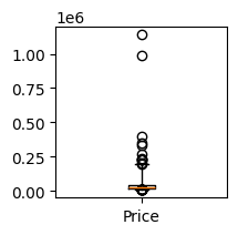
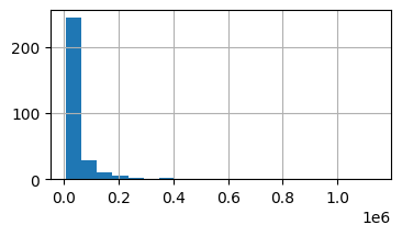
The Price variable has a long tail as can be seen from its adjusted boxplot and its histogram. It’s a good idea to apply a power transformation to it to make it more symmetric.
[8]:
adjusted_boxplot(clean_data['Price'],figsize=(2,2))
[8]:
[Boxplot(median=26505.0, q1=18902.5, q3=44252.5, upper_whisker=191797.28737567586, lower_whisker=12666.161330745548)]
[9]:
clean_data['Price'].hist(bins=20, figsize=(4,2))
[9]:
<Axes: >
[10]:
price_transformer = RobustPowerTransformer(method='auto').fit(clean_data['Price'])

clean_data['Price_transformed'] = price_transformer.transform(clean_data['Price'])
We can inspect which method was selected as well as which lambda value was applied for the transformation:
[11]:
price_transformer.method, price_transformer.lambda_rew
[11]:
('boxcox', -0.42354039562300644)
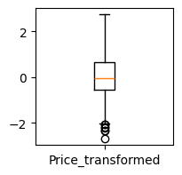
[12]:
adjusted_boxplot(clean_data['Price_transformed'],figsize=(2,2))
[12]:
[Boxplot(median=-0.03153400648124502, q1=-0.5679781382767539, q3=0.6485562387582648, upper_whisker=2.7449937256642296, lower_whisker=-2.0160158561602897)]
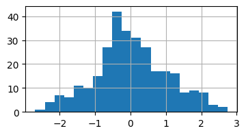
[13]:
clean_data['Price_transformed'].hist(bins=20, figsize=(4,2))
[13]:
<Axes: >
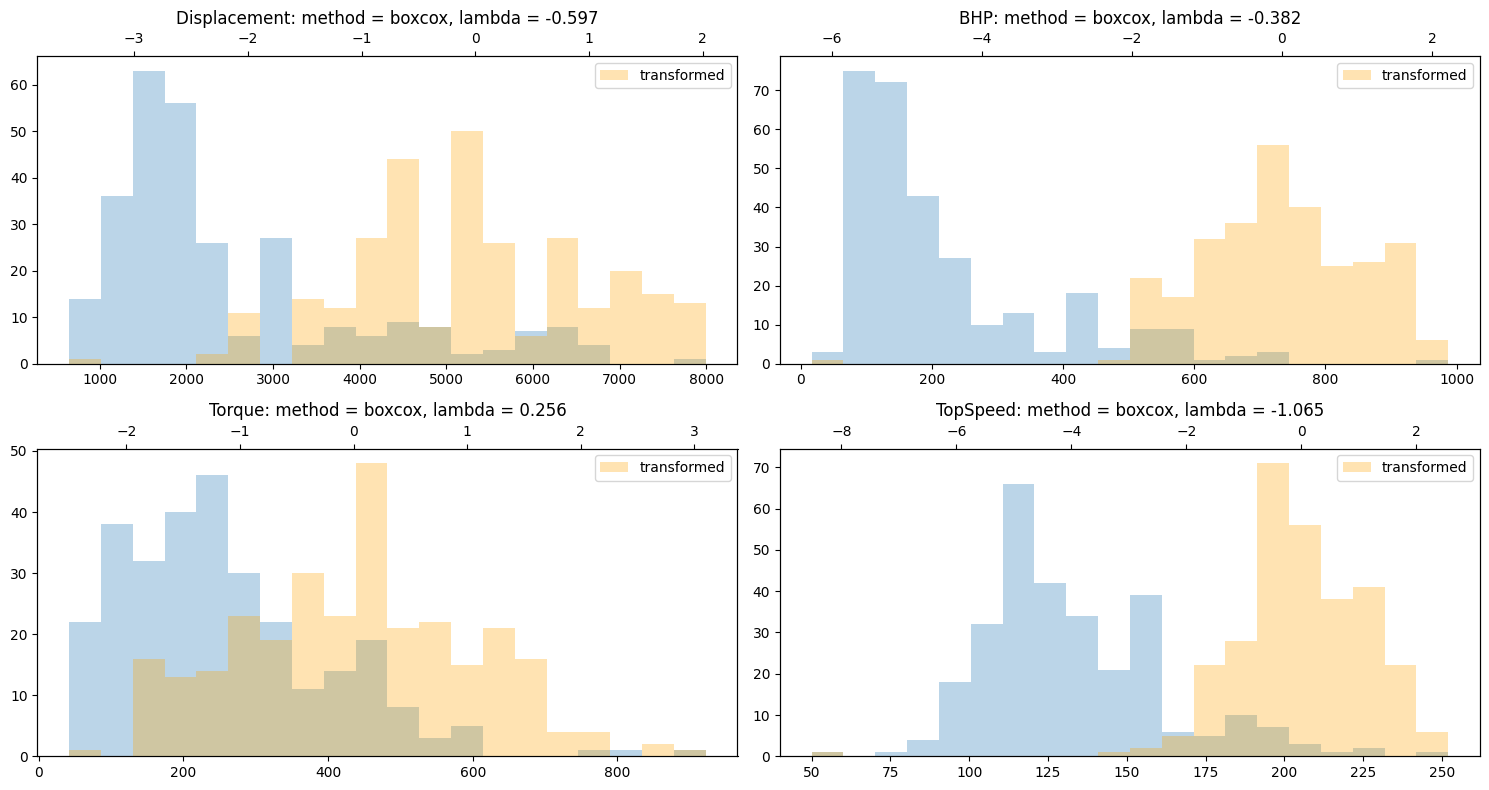
It’s best to also transform displacement, HP, Torque and Topspeed as these variables are also skewed.
[14]:
fig, axs = plt.subplots(2, 2, figsize=(15, 8))
for col, ax in zip(['Displacement', 'BHP', 'Torque', 'TopSpeed'], axs.flatten()):
    clean_data[col].hist(ax=ax, bins=20, alpha=0.3)
    transformer = RobustPowerTransformer(method='auto').fit(clean_data[col].dropna())
    clean_data.loc[~np.isnan(clean_data[col]), col] = transformer.transform(clean_data[col].dropna())
    ax2=ax.twiny()
    clean_data[col].hist(ax=ax2, bins=20, label='transformed', color='orange', alpha=0.3)
    ax.grid(False)
    ax2.grid(False)
    ax2.legend(loc='upper right')
    ax.set_title(f'{col}: method = {transformer.method}, lambda = {transformer.lambda_rew:.3f}')
fig.tight_layout()
Dropping NA
Some methods require the data to be entirely NA free.
[15]:
clean_data2 = clean_data.dropna()
Covariance
First we study the covariance of the dataset by calculating a robust covariance matrix on the numeric features.
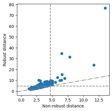
MCD: Minimum Covariance Determinant
[16]:
mcd = FastMCD().fit(clean_data2.drop(columns=['Price']))
[17]:
fig = mcd.distance_distance_plot()
OGK: Orthogonalized Gnanadesikan-Kettenring covariance
We can do the same analysis with other robust covariance estimators, e.g. the OGK covariance:
[18]:
ogk = OGK().fit(clean_data2.drop(columns=['Price']))
[19]:
fig = ogk.distance_distance_plot()
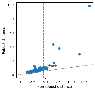
Let’s have a look at the point that seems to lie very far from the majority of the data:
[20]:
data.data.loc[
    clean_data2.index[(ogk._robust_distances > 80) & (ogk._mahalanobis_distances > 12)],
    ['Make', 'Model'] + list(set(clean_data2.columns).intersection(set(data.data.columns)))
]
[20]:
| Make | Model | Price | Torque | Displacement | BHP | Acceleration | Height | Length | TopSpeed | Weight | MPG | Width | |
|---|---|---|---|---|---|---|---|---|---|---|---|---|---|
| 41 | BMW | i3 | 33830.0 | 184.0 | 647.0 | 170.0 | 7.9 | 1578.0 | 3999.0 | 93.0 | 1315.0 | 470.0 | 1775.0 |
CellMCD
A robust covariance estimator that can handle missing values is the CellMCD. For more details, we refer to the separate notebook on this topic.
PCA
Next, we apply a well-known robust PCA method to the data, specifically ROBPCA. As the variables of interest have different measurement units and different scales, we first scale the data.
[21]:
scaled_data = RobustScaler(with_centering=False).fit_transform(clean_data2.drop(columns=['Price']))
pca = ROBPCA().fit(scaled_data)
[22]:
score_distances, orthogonal_distances, score_cutoff, od_cutoff = pca.plot_outlier_map(scaled_data, return_distances=True)
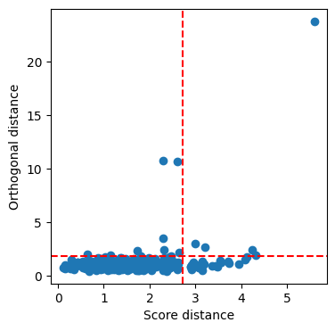
We can inspect the bad leverage points:
[23]:
data.data.loc[
    clean_data2.loc[(score_distances > score_cutoff) & (orthogonal_distances > od_cutoff)].index,
    ['Make', 'Model'] + list(set(clean_data2.columns).intersection(set(data.data.columns)))
]
[23]:
| Make | Model | Price | Torque | Displacement | BHP | Acceleration | Height | Length | TopSpeed | Weight | MPG | Width | |
|---|---|---|---|---|---|---|---|---|---|---|---|---|---|
| 41 | BMW | i3 | 33830.0 | 184.0 | 647.0 | 170.0 | 7.9 | 1578.0 | 3999.0 | 93.0 | 1315.0 | 470.0 | 1775.0 |
| 49 | Bugatti | Veyron | 1139985.0 | 922.0 | 7993.0 | 987.0 | 2.5 | 1204.0 | 4462.0 | 252.0 | 1990.0 | 10.0 | 1998.0 |
| 135 | Land Rover | Defender | 28195.0 | 265.0 | 2198.0 | 122.0 | 14.7 | 1790.0 | 4785.0 | 90.0 | 2120.0 | 25.0 | 1790.0 |
| 164 | Mercedes-Benz | G-Class | 82945.0 | 398.0 | 2987.0 | 211.0 | 9.1 | 1951.0 | 4662.0 | 108.0 | 2500.0 | 25.0 | 1760.0 |
| 196 | Pagani | Huayra | 990000.0 | 811.0 | 5980.0 | 730.0 | 3.3 | 1169.0 | 4605.0 | 230.0 | 1350.0 | 23.0 | 2036.0 |
Outlier detection
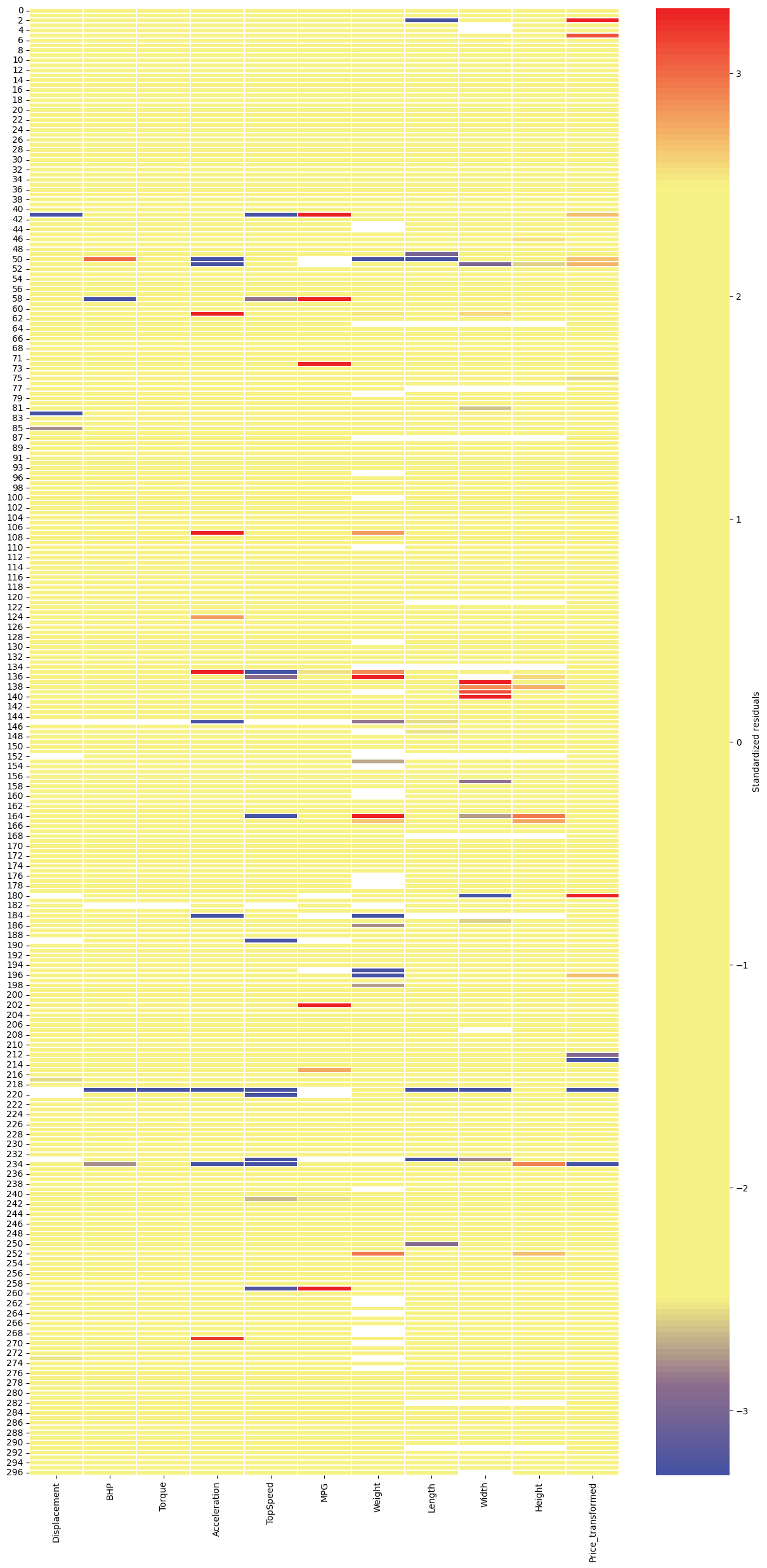
We can also detect cellwise outliers with the DDC estimator. Here we can use the data with NAs, as DDC can handle missing values.
[24]:
ddc = DDC().fit(clean_data.drop(columns=['Price']))
[25]:
ddc.cellmap(clean_data.drop(columns=['Price']), figsize=(15,30))
[25]:
<Axes: >
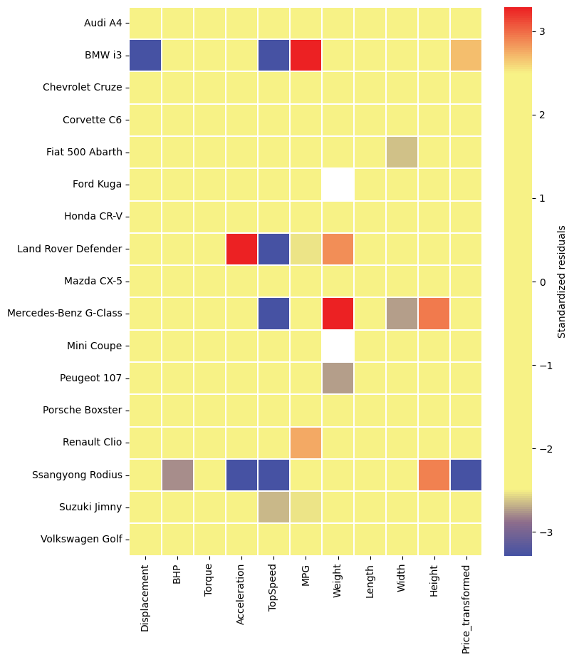
[26]:
row_indices = np.array([ 11,  41,  55,  73,  81,  94,  99, 135, 150, 164, 176, 198, 209,
       215, 234, 241, 277])
ax = ddc.cellmap(clean_data.drop(columns=['Price']), figsize=(8,10), row_zoom=row_indices)
cars = data.data.apply(lambda row: f"{row['Make']} {row['Model']}", axis=1).tolist()
ax.set_yticklabels([cars[i] for i in row_indices], rotation=0);
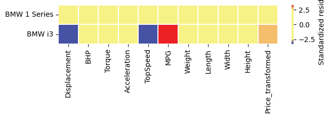
We can additionally zoom in on 2 BMWs:
[27]:
ax = ddc.cellmap(clean_data.drop(columns=['Price']),row_zoom=[31,41], figsize=(7,1))
ax.set_yticklabels([cars[i] for i in [31,41]], rotation=0);
total flagged cells:
[28]:
ddc.cellwise_outliers_.sum()
[28]:
88
DDC also predicts rowwise outliers:
[29]:
clean_data.loc[ddc.predict(clean_data.drop(columns=['Price']), rowwise=True)]
[29]:
| Price | Displacement | BHP | Torque | Acceleration | TopSpeed | MPG | Weight | Length | Width | Height | Price_transformed | |
|---|---|---|---|---|---|---|---|---|---|---|---|---|
| 50 | 44995.0 | 0.219169 | 0.701029 | -0.220938 | 3.1 | 0.921638 | NaN | 575.0 | 3300.0 | 1685.0 | 1140.0 | 0.668256 |
| 51 | 22995.0 | -0.569636 | -0.524540 | -1.071051 | 5.9 | -0.748566 | NaN | 550.0 | 3380.0 | 1575.0 | 1115.0 | -0.247651 |
| 61 | 30245.0 | 0.613284 | 0.109823 | 0.297162 | 12.8 | -0.590064 | 35.0 | 2305.0 | 5218.0 | 1998.0 | 1818.0 | 0.157953 |
| 124 | 25995.0 | 0.613284 | 0.276559 | 0.782252 | 12.9 | -1.033160 | 34.0 | 2075.0 | 4223.0 | 1873.0 | 1840.0 | -0.060330 |
| 135 | 28195.0 | 0.161107 | -0.571367 | 0.297162 | 14.7 | -2.246128 | 25.0 | 2120.0 | 4785.0 | 1790.0 | 1790.0 | 0.058518 |
| 145 | 36200.0 | NaN | NaN | NaN | 0.0 | NaN | NaN | 876.0 | 3785.0 | 1850.0 | 1117.0 | 0.399504 |
| 180 | 29045.0 | NaN | -1.988366 | -0.920764 | 15.9 | -2.161801 | NaN | 1110.0 | 3475.0 | 1475.0 | 1610.0 | 0.100958 |
| 184 | 30000.0 | -0.075638 | -0.775908 | -1.348513 | 4.5 | -0.344059 | NaN | 490.0 | NaN | NaN | NaN | 0.146581 |
| 219 | 6950.0 | NaN | -6.267469 | -2.504821 | 0.0 | -8.518526 | NaN | 450.0 | 2337.0 | 1237.0 | 1461.0 | -2.690158 |
| 234 | 17995.0 | -0.042303 | -0.128325 | 0.297162 | 0.0 | -1.154841 | 38.0 | 2059.0 | 5125.0 | 1915.0 | 1845.0 | -0.652657 |
Finally, DDC can impute missing data:
[30]:
ddc.impute(clean_data.drop(columns=['Price'])).loc[ddc.predict(clean_data.drop(columns=['Price']), rowwise=True), :].style.format('{:.2f}')
[30]:
| Displacement | BHP | Torque | Acceleration | TopSpeed | MPG | Weight | Length | Width | Height | Price_transformed | |
|---|---|---|---|---|---|---|---|---|---|---|---|
| 50 | 0.22 | -0.04 | -0.22 | 8.61 | 0.92 | 41.83 | 1364.54 | 4331.18 | 1685.00 | 1140.00 | -0.26 |
| 51 | -0.57 | -0.52 | -1.07 | 11.65 | -0.75 | 55.07 | 550.00 | 3380.00 | 1722.44 | 1482.87 | -1.19 |
| 61 | 0.61 | 0.11 | 0.30 | 7.88 | -0.59 | 35.00 | 2305.00 | 5218.00 | 1869.97 | 1818.00 | 0.16 |
| 124 | 0.61 | 0.28 | 0.78 | 8.73 | -1.03 | 34.00 | 2075.00 | 4223.00 | 1873.00 | 1840.00 | -0.06 |
| 135 | 0.16 | -0.57 | 0.30 | 9.85 | -0.23 | 25.00 | 1483.18 | 4785.00 | 1790.00 | 1790.00 | 0.06 |
| 145 | 0.21 | 0.49 | 0.12 | 8.79 | 0.87 | 36.24 | 1515.46 | 3785.00 | 1850.00 | 1117.00 | 0.40 |
| 180 | -1.54 | -1.99 | -0.92 | 15.90 | -2.16 | 65.02 | 1110.00 | 3475.00 | 1693.47 | 1610.00 | -1.91 |
| 184 | -0.08 | -0.78 | -1.35 | 11.16 | -0.34 | 50.55 | 1391.73 | 4163.08 | 1757.12 | 1447.99 | 0.15 |
| 219 | -1.47 | -1.12 | -1.12 | 15.50 | -0.61 | 58.45 | 450.00 | 3667.15 | 1654.07 | 1461.00 | -0.89 |
| 234 | -0.04 | 0.56 | 0.30 | 9.32 | 0.50 | 38.00 | 2059.00 | 5125.00 | 1915.00 | 1428.56 | 0.63 |
Regression
We can use robust regression to predict the (transformed) price using the remaining variables. For regression, we again have to drop all missings.
[31]:
X = clean_data2.drop(columns=['Price', 'Price_transformed'])
y = clean_data2['Price_transformed']
As an example, we use the MM-estimator of regression:
[32]:
estimator = MMRegression().fit(X, y)
estimator.model.coef_
[32]:
array([ 2.71338919e-01,  4.24224370e-01,  2.04835077e-01,  3.63925688e-02,
        8.75191584e-02,  3.77330897e-03,  4.65624836e-04, -2.97257613e-04,
        8.37238866e-04, -9.42993337e-04])
We can now get a diagnostic plot and ask for the underlying data
[33]:
resid, std_resid, distances, vt, ht = estimator.outlier_map(X, y.to_numpy(), return_data=True)
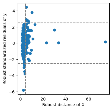
Now we can get an overview of the bad leverage points:
[34]:
bad_leverage_idx = (np.abs(std_resid) > vt) & (distances > ht)
data.data.loc[
    clean_data2[bad_leverage_idx].index, ['Make', 'Model', 'Price']
].assign(predicted_price=price_transformer.inverse_transform(estimator.predict(X.loc[bad_leverage_idx])).round())
[34]:
| Make | Model | Price | predicted_price | |
|---|---|---|---|---|
| 2 | Aston Martin | Cygnet | 30995.0 | 15326.0 |
| 5 | Aston Martin | V12 Zagato | 396000.0 | 117938.0 |
| 164 | Mercedes-Benz | G-Class | 82945.0 | 34576.0 |
| 222 | Rolls-Royce | Phantom | 352720.0 | 116166.0 |
| 223 | Rolls-Royce | Phantom Coupe | 333130.0 | 111003.0 |
| 253 | Toyota | Prius | 24045.0 | 16272.0 |